Project
Report—A Simple 2-D Cloud Model with a Parameterized Ice-Phase Microphysics
Summary:
The simulation results of the tropical convection are
reported by a simple 2-D cloud model with a Parameterized Ice-Phase
Microphysics.
The growing and mature stages
of the convection can be seen from the simulation results. As a comparison, the
moist convection is also modeled using liquid water only microphysical
parameterizations. For the simulation with ice microphysics, the kinetic energy
is a little bigger than that without ice, to due the latent heating by melting
of ice hydrometeors. However, the vertical velocity fields, perturbation of
potential temperature fields and the non-dimensional perturbation pressure
fields are very similar for the simulations with and without ice microphysical
processes.
Model
The model is based on the
quasi-compressible outflow model (QCOM) described in Droegemeier and Wilhelmson
(1987). Ice or water only microphysical processes are added by following Lord
et al (1984). The model predicts the horizontal velocity (v), the vertical
velocity (w), the potential temperature (![]() ) and the non-dimensional perturbation pressure (
) and the non-dimensional perturbation pressure (![]() ). The equations in Cartesian coordinates (y,z) are:
). The equations in Cartesian coordinates (y,z) are:
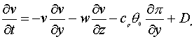 (1)
(1)
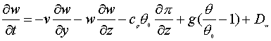 (2)
(2)
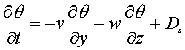 (3)
(3)
 (4)
(4)
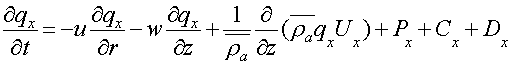 (5)
(5)
where ![]() in Eq.(4) is the constant sound speed. In Eq.(5), q is mixing
ratio, the subscript x denotes water vapor, cloud water, rain, cloud ice, snow
and graupel.
in Eq.(4) is the constant sound speed. In Eq.(5), q is mixing
ratio, the subscript x denotes water vapor, cloud water, rain, cloud ice, snow
and graupel. ![]() is the
height-dependent basic-state density of air. U is the mass-weighted fall speed
(U>=0) for precipitating particles, P the net production rate due to the
bulk-parameterized microphysical processes, C the source or sink of cloud water
and cloud ice due to condensation, deposition, evaporation and sublimation, and
D is eddy diffusion. (For the details of the microphysical processes in the
model, see Lord et al. 1984)
is the
height-dependent basic-state density of air. U is the mass-weighted fall speed
(U>=0) for precipitating particles, P the net production rate due to the
bulk-parameterized microphysical processes, C the source or sink of cloud water
and cloud ice due to condensation, deposition, evaporation and sublimation, and
D is eddy diffusion. (For the details of the microphysical processes in the
model, see Lord et al. 1984)
The simple eddy viscosity approach is used
for turbulence closure. The lower and upper boundaries are both rigid and free
slip. The lateral boundary conditions are periodic. The domain extends 30 km
horizontally and 15 km vertically. The vertical resolution is 100 m, the
horizontal resolution is 200 m. Time step is 0.1 s.
The GATE mean sounding (Fig. 1) is used as the background sounding. For
initializing convection, a warm bubble (Fig. 2) is
added.
Results: (at 6000s
simulation)
a.
Simulation
of a tropical convection with ice-microphysics processes: (with ice, including
cloud water, rain water, cloud ice, snow, and graupel)
Animation1:
Time series of the contours of hydrometeor mixing ratios
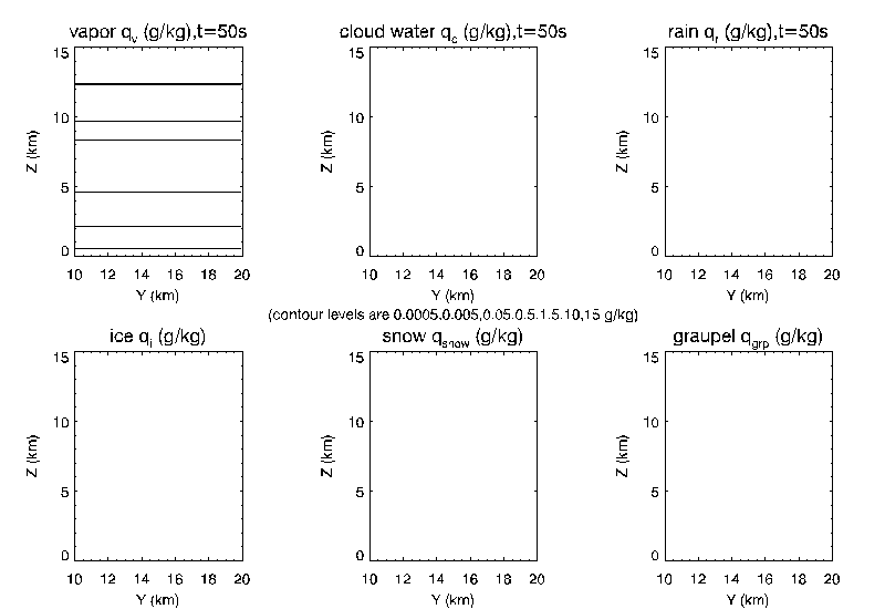
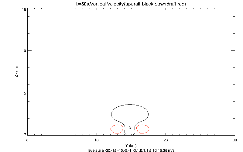
Animation2:
Time series of the contours of vertical velocity
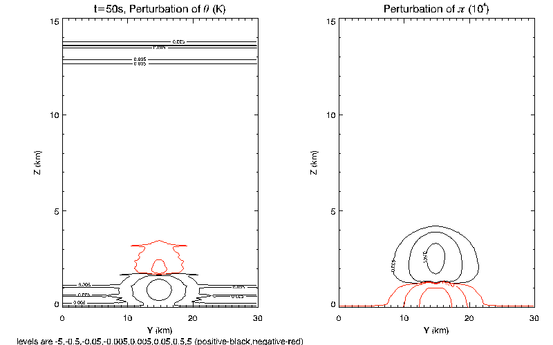
Animation3:
Time series of the contours of potential temperature perturbation and the
non-dimensional perturbation pressure.
b.
Simulation of a tropical convection with
ice-microphysics processes (without ice, including cloud water and rain water):
Animation4: Time
series of the contours of hydrometeor mixing ratios
Animation5: Time
series of the contours of vertical velocity
Animation6:
Time series of the contours of potential temperature perturbation and the
non-dimensional perturbation pressure.
c.
Comparison
of the results with ice and without ice:
Fig3(jpg) or (PDF) : The kinetic
energy with and without ice vs. time.
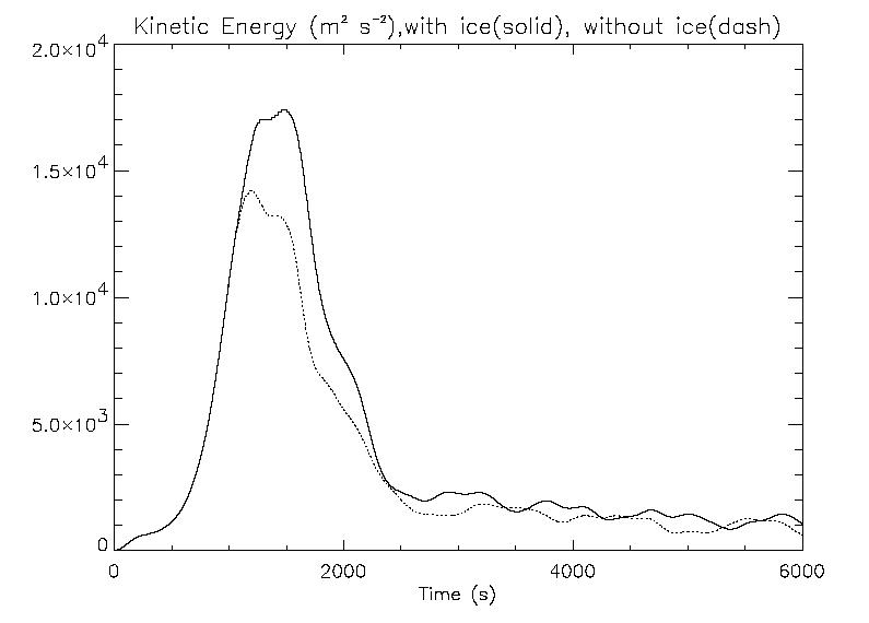
Fig4: Time series of domain average mixing ratios
of each hydrometeor species for the simulation with ice (a) and without ice
(c).
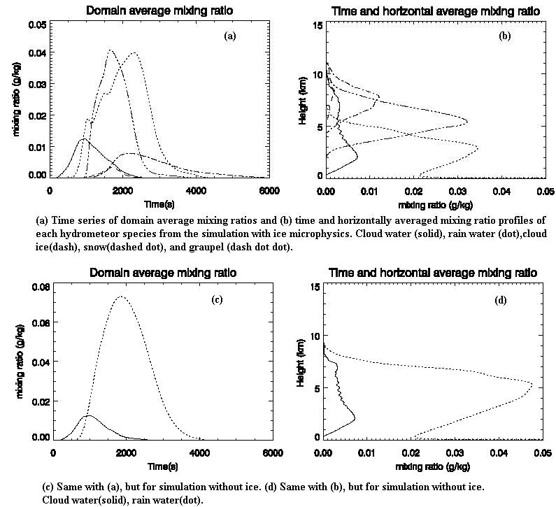
Time and horizontally
averaged mixing ratio profiles of each hydrometeor species with ice (b) and
without ice (d).
Fig5:
Time series of maximum mixing ratios for each hydrometeor species for the
simulation with ice.
Fig6:
Time series of maximum mixing ratios for each hydrometeor species for the
simulation without ice.
Fig7:
Time series of maximum and minimum of perturbation of ![]() , perturbation of
, perturbation of ![]() , vertical velocity, and horizontal velocity for the
, vertical velocity, and horizontal velocity for the
simulation with ice.
Fig8:
Time series of maximum and minimum of perturbation of ![]() , perturbation of
, perturbation of ![]() , vertical velocity, and horizontal velocity for the
, vertical velocity, and horizontal velocity for the
simulation with ice.
Possible future simulation:
To simulate a squall line by adding a wind shear at initial conditions.