Atmos 5210: Term Project
Objectives
After completing this project, students should be able to:
- Perform fine-scale frontal analysis using high-density sufrace observations in complex terrain.
- Identify fronts in high-resolution, short-range forecasts and subjectively evaluate the capabilities and limitations of those forecasts.
- Diagnose and describe the three-dimensional structure of cold fronts and associated precipitation features using high-resolution gridded analyses.
- Recognize that there are frontal precipitation archetypes beyond those depicted by the Norwegian Cyclone Model.
Introduction
On 27 November 2017, a strong surface cold front moved across northern Utah and was surveyed by the Doppler on Wheels, which was deployed on the Stansbury Island Causeway. Forecast issues prior to deployment included the timing of frontal passage and the onset of precipitation. Here, we take a closer look at the structure of that event and the performance of forecasts leading up to it.
Part I
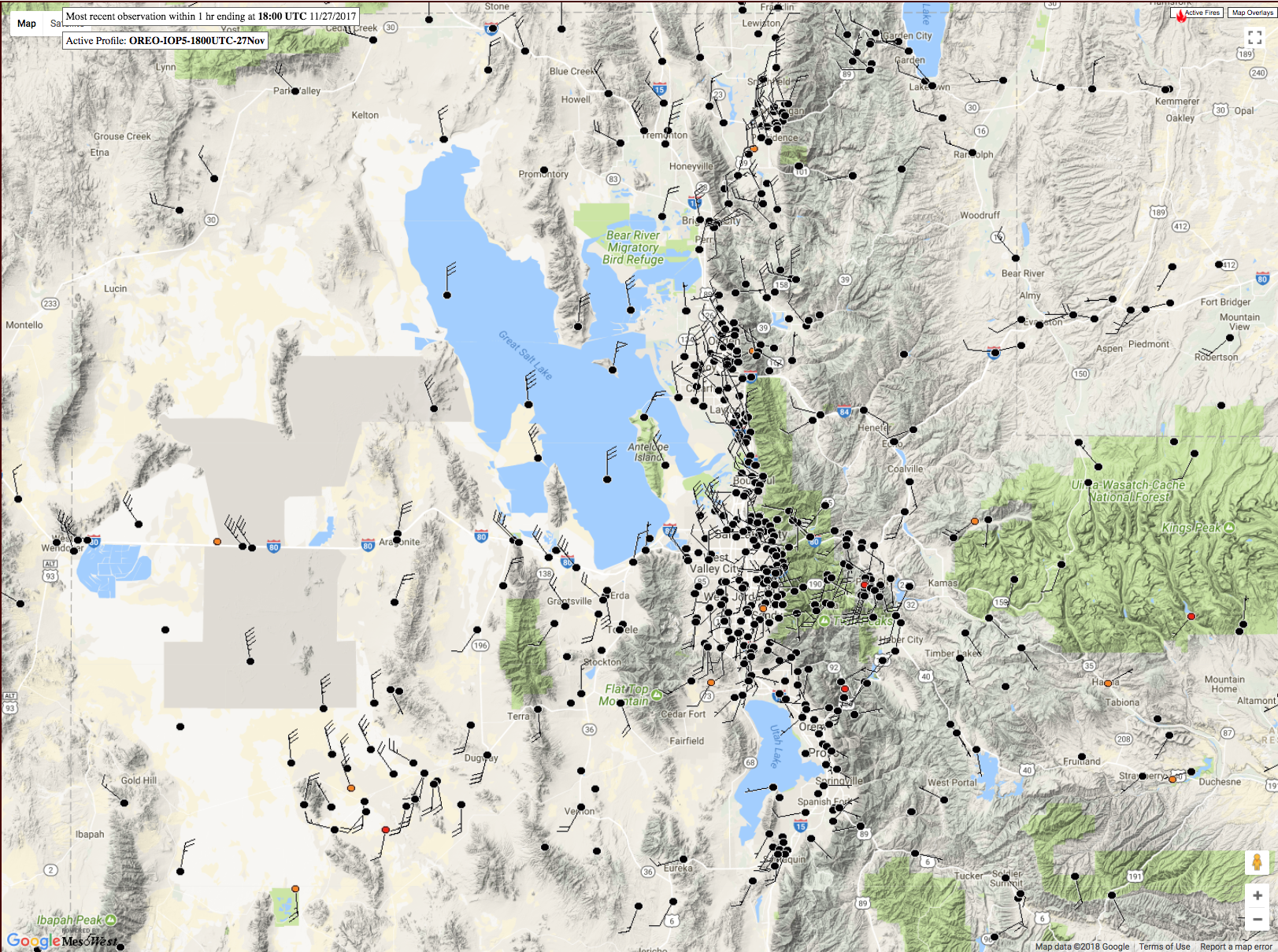
Click here to access a MesoWest plot for 1800 UTC 27 November 2017. Place the image into powerpoint and analyze the position of the front across northern Utah. Use the clickable mesowest plot available here to access the MesoWest data at this time (it may take a minute or two to load), examine temperatures, and examine point-clickable graphical and tabular time series to fine-tune the frontal position and check observation times (note that some data on this map may be an hour old and that can be important for detailed analysis). Pay careful attention to detail.
Using the hyperlinks in this paragraph, dowload and add to powerpoint slides with the the 0300, 0600, 0900, 1200, 1500 UTC initialized HRRR forecasts valid at 1800 UTC 27 November. Identify the front in each of these forecasts (note: you will need to do this based entirely on the wind).
Answer the following questions:
- How large are the errors in front position in each HRRR forecast?
- How do these errors change with decreasing forecast lead time? Explain these changes.
- What are some of the potential ramifications for such errors for forecast customers?
Part II:
Login to an imac in 711 WBB, start IDV, and open the bundle 5210 -> Oreo-iop5-18zHRRR-3Dfront. This will bring up an analysis from the HRRR combined with KMTX radar reflectivity at 1800 UTC 27 November 2017. Give it a few moments to load in. Everything you need to complete this project should be available in the right-hand legend including:
- 3-D isosurfaces of Rain+Snow Mixing Ratio (defaults to 4x10⁻⁴ kg/kg), potential temperature (298 K), and topography.
- Plan views of the potential temperature (850 hPa), horizontal temperature gradient magnitude (850 mb), and horizontal frontogenesis (850 mb and 700 mb).
- Wind vectors at 10 m and 850 mb
- Contours of surface (2-m) potential temperature on the topography as a 3-D surface.
- Vertical profiles of RH and wind.
- Cross sections of horizontal frontogenesis, meridional wind, and potential temperature.
- Lowest-tilt radar reflectivity from the KMTX radar.
You can toggle these products on and off, use IDV to change the levels of the plan view analyses, move the cross sections and probes, and navigate the image three dimensionally. Take soem time to orient yourself to the frontal and precipitation structure at this time.
Using the bundle address the following:
- Based on a comparison of the 2-m and 850-mb potential temperature analyses, how does the position and strength of the front (as inferred from the distance between the isentropes) change with height just above the surface? How does this compare with your expectations?
- Based on insepction of the 850-mb potential temperature, temperature gradient magnitude, frontogenesis and vector wind analyses, where geographically is the front strongest (in terms of the temperature gradient) and is this consistent with the frontogenesis? Based on the winds, can you explain how the frontogenesis changes in strength along the front?
- Position the vertical cross sections from N-S through the Tooele Valley and perpendicular to the front. How does the frontal depth, frontogenesis, and struture of the post-frontal northerly flow vary as one moves northward into the post-frontal airmass? Include some annotated images to make your point. You may find the potential temperature isosurface to be helpful.
- Drag the vertical wind profile from south to north along the cross section, across the front, and into the post-frontal airmass. How does the vertical profile of winds change as one moves across the front toward the cold air and then further north into the post-frontal environment?
- Do some investigating and explain why the precipitation band lags the surface front, in contrast to what one might expect from the cold front depiction provided by the Norwegian Cyclone Model. Provide some images and an explanation to support your hypothesis.
Part III
Click here to download a powerpoint containing a sequence of DOW radar reflectivity and Doppler velocity (green towards, red away) velocity images (RHIs) taken through the cold front as it pushed across the northern Tooele Valley toward the Oquirrh Mountains from 1728 UTC to 1745 UTC, just prior to the tima analyzed previously.
For each time, analyze the position of the leading portion of the front on both the doppler velocity and radar reflectivity images, as well as indicating the position of the front at the surface along the indicated RHI position in the upper-right hand panel.
Answer the following questions:
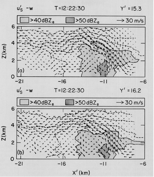
How well does the Doppler velocity structure match that found by Carbone (1982) for a frontal case in California and available here.
Where is the radar reflectivity maximum relative to the frontal surface and does this make sense based on the Doppler velocity analysis? Explain your answer?
What is the speed of the front (km/hour). Does it appear to move at constant speed as it approaches the Oquirrh or is there evidence of acceleration or decelleration?